MineExpress CS 175: Project in AI (in Minecraft) - Group 8 Herobrine
Video
Project Summary
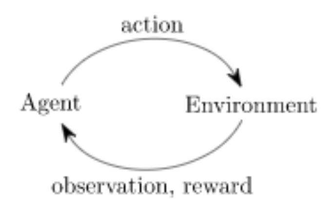
MineExpress is an Artificial Intelligence project developed for routing or delivery tasks, like amazon shipping, Uber, or UberEat. Our goal is to train our agents to pick up and drop off packages or food to the right places. At the same time, we aim to find an optimal path to navigate our agent to those places. To achieve this, we utilized three methods: q-learning algorithm, Dijkstra’s algorithm, and random action. Q-learning is our main algorithm. It utilized an agent-environment loop shown below. Within each process, the agent chooses an action, and the environment returns an observation and rewards. We will visualize this process of learning in the game Minecraft and Malmo platform.
The mission is inspired by TSP (Traveling Salesman Problem), and we also reference the taxi-v3 environment from Gym (OpenAI) by stimulating the same game settings where our agent has pickup and drop-off actions.
Motivation:
During the pandemic of the covid-19, many people stayed at home to ensure their safety. At this time, food and express delivery often face the problem of insufficient manpower. An AI that can adapt to any environment and perform such work can greatly facilitate people’s lives. We hope to develop such AI that can deliver packages correctly with low time consumption. Since the situation is more complex than the simulation in the real world, using Reinforcement Learning algorithms is essential because it allows our agents to learn from and adapt to any new environment. For example, a pizza delivery AI wants to deliver the food to a new neighborhood. AI/ML algorithms allow the AI to learn human intervention. Also, in our study, we are trying to apply reinforcement learning algorithms to the pathfinding problem to demonstrate the feasibility of reinforcement learning algorithms in this field which is commonly solved by mathematical machine learning algorithms.
Environment Settings:
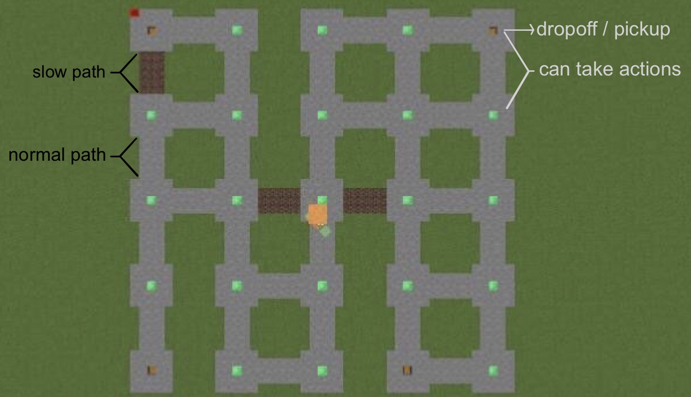
The figure above shows our training environment. The arena is 45 * 45 with 25 possible locations where our agent can make an action. This location either has a green block or a chest (brown block) in the center. It also has 4 possible locations that are valid for pickup or drop-off. These locations have a chest in the center. At the beginning of each mission, one of the four location that have a chest will be assigned as the package location for pickup, and one of the remaining three locations will be assigned as the destination for drop-off. Our agent should only pick the package up at the package location and drop it off at the destination. There are two types of the path. It simulates the real-world environment with different moving speeds for routes. The stone blocks are the path with normal speed. The soul sand block, however, slows down the speed of our agent.
Our agent will start randomly in one of the 25 locations.
Block Types summary:
- Normal state: Emerald Block
- Pickup / Drop-off state: Chest
- Common Speed: Stone
- Speed Down: Soul Sand
Approaches
Setting For All Approaches
Actions:
We use discrete movement commands to train our agents because using continuous movement will make it harder to determine the q-value for an individual state. There are 6 possible actions in a state:
0: move north
1: move south
2: move east
3: move west
4: pickup
5: drop-off
Rewards:
- Pass the soul sand path (that slows down the agent’s speed): -4
- Pass the stone path (with normal speed): -1
- Pick up the package in the wrong location: -10
- Drop off the package in the wrong location: -10
- Drop off the package in the right location: +20
Malmo XML does not support any of the above reward settings. Because the dropoff location is only valid to drop-off when the package has picked up, and because the pickup location will no longer be valid to pick up after the package has picked up, the validity of these blocks changes when a mission is running. The built-in reward element
We self-defined all the rewards. We store the previous block type, look it up when summing rewards, and update it in each iteration to reward for passing different types of blocks. To determine the validity of each block to pick up and drop off, we store the pickup and dropoff location as a class variable. When the action pickup is executed, we check if the package has not been picked up and the pickup location matches the current agent location. if the condition fails, we reward negatively. Similarly, when the action drop-off is executed, we check if the package is carried by the agent and two locations match.
Algorithms
Random Action
We use random actions to be the baseline of the q-learning algorithm. It simply chooses one of the 6 actions at each state.
Dijkstra’s Algorithm
We use Dijkstra’s algorithm as the upper bound for the q-learning algorithm because Dijkstra’s algorithm can always find the overall optimal path with enough information about the environment. We use the same discrete movement commands and action list as the q-learning algorithm for comparison.
To find the optimal path from a start point to destination, we use Dijkstra’s algorithm in following steps:
(1. Initialize two priority dictionaries and save the start point)
grid_dist[ {key=block index}: {value=cost from the start to the key} ]
pre_dist [ {key=block index}: {value=neighbor block index that constitutes the current optimal path from start to the key} ]
grid_dist[source] = 0
pre_dist[source] = -1

(2. Add path to pre_dist)
While grid_dist is not empty:
	Choose a key k with the smallest value from grid_dist
	If any of the k’s neighbor blocks is valid:
		Determine the cost from start to the block (start to k + k to block)
		If block index not in grid_dist or cost < old value:
			Update grid_dist[block_index] = cost
			Update pre_dist[block_index] = k
		Delete k from grid_dist

(3. Extract the path from pre_dist)
curr = destination
while pre_dist[curr] != -1:
	Add curr to the beginning of optimal_path_list
	curr = pre_grids[curr]
Add the start point to the beginning of optimal_path_list
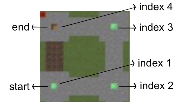
For example, we want to find an optimal path from block 1 to block 4 showing above, grid_dist and pre_dist will undergo the following changes:
Before Iteration:
	grid_dist[ 1:0 ]
	pre_dist[ 1:-1 ]
Iteration 1:
	grid_dist[ 2:1, 4:4 ]
	pre_dist[ 1:-1, 2:1, 4:1 ]
Iteration 2:
	grid_dist[ 3:2, 4:4 ]
	pre_dist[ 1:-1, 2:1, 4:1, 3:2 ]
Iteration 3:
	grid_dist[ 4:3 ]
	pre_dist[ 1:-1, 2:1, 4:3, 3:2 ]
Iteration 4:
	grid_dist[]
	pre_dist[ 1:-1, 2:1, 4:3, 3:2 ]
End
The above pre_dist provides us the optimal_path_list = [1, 2, 3, 4]. Once we get this path_list, we can navigate our agent to finish the mission.
For rewards, we go through the optimal_path_list. If the block is stone, we minus 1 to the reward; if the block is soul sand, we minus 4 to the reward. The reward is added to 20 when the mission ends.
Q-Learning Algorithm
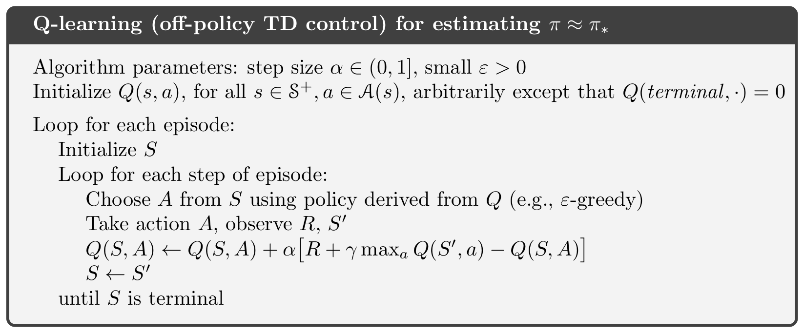
The Q-learning algorithm learns through the following series of actions: observes the environment, takes the best actions, measures the rewards, and updates the q-table.
Q-table:
Our q-table has 500 states (5 * 5 * 5 * 4). 25 possible locations for the agent, 4 possible source locations for the package, and 4 possible locations for the destination. Also, since our agent has to pick up the package before delivering it to the designation;and it is not reasonable for the agent to finish the mission before picking up the package. We also need to consider the difference between pickup and delivery state. Therefore, there are 5 possible package locations since the package may be any of the four chests or inventory slot of the agent. And, we encode all the information into one state number to show our agent different state as the observation. The state number range is from 0 to 499.
We store the q-table in a 2-dimensional NumPy array, with 500 rows and 6 columns. Each row represents a state, and each column represents an action at the specific state. With 500 states and 6 possible actions in each state, our q-table stores a total of 3000 q-values.
Update Q-Value:
Initially, all q-values in the q-table are 0. After an action is executed, We store the previous state into the q-table and update the q-value for the action. The q-value is determined by the equation below:

α: learning rate (range from 0 to 1)
γ: discount rate for future rewards (range from 0 to 1)
Good choices of α and γ are important to the performance of our agent. For example, setting α to 0.1 and γ to 0.99 makes the agent stick to a feasible but non-optimal path. We finally set α to 0.7 and γ to 0.618 after some tests.
Q(s, a) : previous state and action
maxQ’(s’, a’): q-value for the best action in the agent's current state
R(s,a): reward after executing the previous action.
For example, if our agent is initialized in the location (0, 0). The package location indexed is 1, and the drop-off location index is 2. An action, such as move south, updates the state 6 (4 * (5 * (5 * 0 + 0) + 1) + 2) and its action space 1, which represent move east. In this case, s’ will be 26 (4 * (5 * (5 * 0 + 1) + 1) + 2); and a’ can be any action because they are all 0 at the beginning of the training.
Next Actions:
A new action is chosen by ε-greedy exploration below.
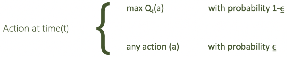

It allows our agent to choose the current best action based on the q-table while ensuring some Randomness of choice to avoid our agent stack at a local optimum. We also apply an exponential decay to the epsilon based on the formula shown in Figure 6, to make the epsilon reduces faster at the beginning and gradually converge at a specific value.
The parameters for epsilon-greedy exploration shows below:
Initial Epsilon(ε_max): 1
Min Epsilon(ε_min): 0.2
Decay Rate(λ): 0.001
Episode(t): 0~4999
Summing up:
the whole process of training our agent by q-learning is shown below:
Comparison between Dijkstra’s algorithm and q-learning:
Dijkstra’s algorithm is easy to implement and can find the optimal solution much faster than q-learning. For our problem, Training our agent with q-learning can take up to a day in the Malmo platform, however, Dijkstra’s algorithm only runs for a few seconds for each mission. If our agent knows how the surrounding environment looks, Dijkstra’s algorithm is more useful than q-learning.
However, for many real-world tasks, the agent is placed in an unfamiliar environment, and Dijkstra’s algorithm will not work. It is because Dijkstra’s algorithm needs to find the path using the environment information before it can make an action. For example, in our problem, we give it full state observation by setting
Evaluation
Quantitative
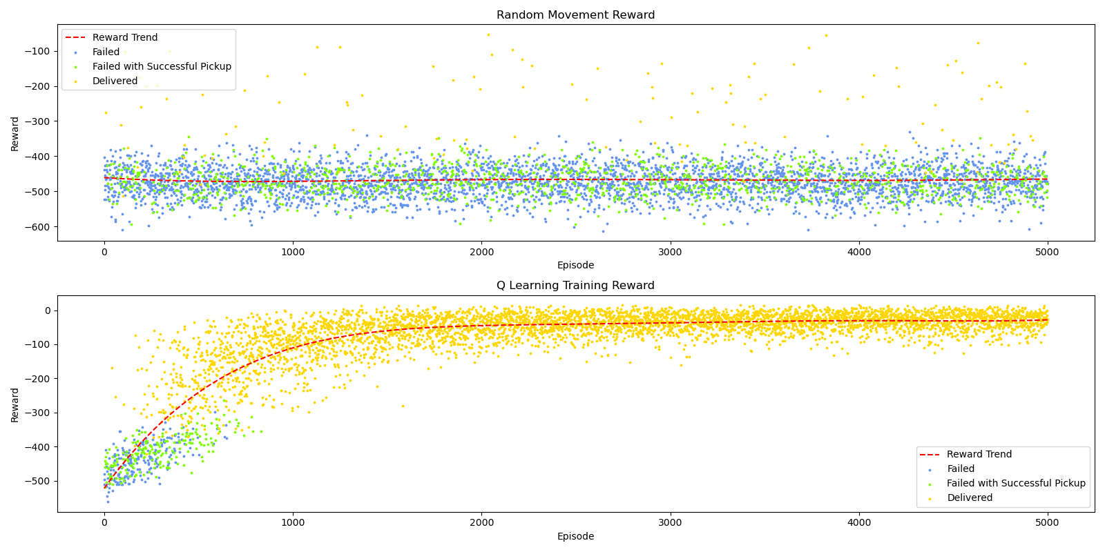
From the figure 8, we can see that the reward trend of the random movement does not have a significant change, but it still has a 2% possibility to get an unexpected successful result, which indicates that the mission with 500 states may not be complex enough. In contrast, the reward trend of the Q-learning agent has a significant logarithmic increment; and the rewards converge at -50 after 2000 episodes. We can also see a clear learning process through the figure. In the beginning, the agent has a high failure rate, since the agent is not familiar with the arena and tries to use random behaviors for exploration. After 500 episodes, We can see that the number of failed missions has been drastically reduced, replaced by more successful missions and failed missions with pickup. Then, after around 900 episodes, the agent can complete almost all missions successfully, but we can still observe a significant increase in reward until 2000 episodes. We also noticed that the variance of the reward after 2000 episodes remains at a high level, we believe that is caused by the high minimum epsilon rate to ensure our agent would not stack in a local optimal.
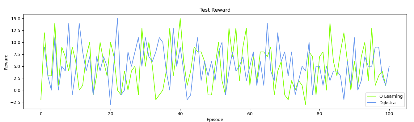
Figure 9 is the test reward comparison between Dijkstra’s algorithm and the q-learning algorithm (after training). In general, we were surprised to find that the average reward of the Dijkstra algorithm and the q learning algorithm is not significantly different. We also found that the variance of the q learning algorithm is much lower than the result in the training reward diagram, which directly proves our previous guess about the correlation between the high variance and epsilon rate.
Qualitative
For qualitative evaluation, we can simply monitor the action, the reaching rate, and the final score of the agent. We will monitor the action of the agent visually to see whether our agent always chooses the best behavior. Also, if the agent has a high reward with a great scale of score improvement, it means that the agent is most likely to choose the better action to reach the goal, which is a perfect indication in the qualitative evaluation.
The video above shows the performance of the random movement and q-learning agent. We can see the random movement agent chooses actions randomly and cannot complete the mission. In contrast, we can see that our well-trained q-learning agent chooses the path that leads to the highest reward. For example, in the first episode, when there is a soul sand path in front of our agent, it will choose to take a detour (take three stone paths) because a soul sand path costs 4, while three stone paths only cost 3. However, in the third episode, our agent also chooses the soul sand path and failed to find the optimal path. We believe that our agent achieves a local optimum during the training, and we may get a better result with a larger minimum epsilon or smaller decay rate.
Further Improvements
-
Adjust the hyper-parameters of the current q-learning agent to avoid the local optimum and get better performance.
-
Increase the complexity of the problem to make the problem more similar to the real situation.
-
Try more reinforcement algorithms, such as DQN, A3C, to solve the problem.
Contribution
-
Jason Li: Research in different RL algorithms; attempt in the q-learning algorithm (not used); write and revise the final report; record videos; update Github page with various visual effects; Collect and record meeting logs.
-
Yachi Lee: Implement Dijkstra algorithm; attempt in the q-learning algorithm; make the slide for the final video; write approach and motivation and revise other parts of the final report; record video; make the sanity check, and the baseline for a status report.
-
Yilong Huang: Implement the q-learning agent, MalmoUtils, MineExpressEnv, MineExpressEnvSimulator; attempt in the deep q-learning agent; write the evaluation and revise other parts of the final report; edit and record videos; data analysis and visualization; implement a demo ppo agent for the status report.